Previous Entry: NumPyro Workshop Next Entry: The Importance of Importance Sampling
Go Back: Statistics Articles Return to Blog Home
import jax.numpy as jnp
import numpyro
import matplotlib.pyplot as plt
import numpy as np
import numpyro.distributions as dist
import jax
There are two domains we might want to generate $\sum x = 0.0$ over:
- With $x\in[-1,1]$
- With $x\in \mathbb{R}$ and distributed over a unit normal, $x\sim\mathcal{N}_{0,1}$
For the first case there are two ways to do this: a simple but less obvious way and a more labrious but easier to interpret way.
- Draw from a dirichilet distribution and subtract off the average
- We don’t know how many samples will be $x>0$ and how many will fall below the zero line, but we can randomize these numbers, $N_1$ and $N_2$ with an equally weighted binomial distribution. Then, knowing that the “mass” (sum) of points either side must be equal, we can draw the values for the $N_{1/2}$ samples and invert the $x<0$ values. There’s the caveat that we need $N_{1/2} > 0$, but this just takes a few tweaks to how we sample them.
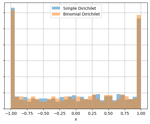
These end up being equivalent (see last fig).
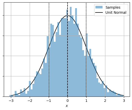
For the continuous domain things are much easier. Draw $N$ samples from a unit normal and subtract off the mean so that they sum to zero. This constrains the values and narrows the overall distribution, and so we need to scale up by a factor $\sqrt{1+\frac{1}{N-1}}$ to get the right variance.
def model_simple(N):
    x = numpyro.sample('x', dist.Dirichlet(jnp.ones(N)))
    x-=X.mean()
    return(x)

def model_cont(N):
    x = numpyro.sample('x1', dist.Normal(0,1), sample_shape=(N,))
    x-=x.sum()/N
    x*=jnp.sqrt(1+1/(N-1))
    return(x)


def model_disc(N):
    N1 = numpyro.sample('N1',dist.Binomial(N-2,0.5)) + 1
    N2 = numpyro.deterministic('N2',N-1-N1) + 1

    if N1>1:
        x1 = numpyro.sample('x1', dist.Dirichlet(jnp.ones(N1)))
    elif N1==1:
        x1 = jnp.array([1.0])

    if N2>1:
        x2 = numpyro.sample('x2', dist.Dirichlet(jnp.ones(N2))) * -1

    elif N2==1:
        x2 = jnp.array([-1.0,])

    return(jnp.concatenate([x1,x2]))
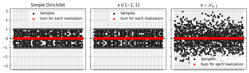
Now testing this for $N=3$ samples over $M=512$ realizations:
N = 3
M = 512
X0 = np.zeros(N*M)
X1 = np.zeros(N*M)
X2 = np.zeros(N*M)
for i in range(M):
    #if i//(M//100)==0: print(i,end='\t')
    with numpyro.handlers.seed(rng_seed=jax.random.PRNGKey(i)):
        X0[i*(N):(i+1)*(N)] = np.array(model_disc(N))
        X1[i*(N):(i+1)*(N)] = np.array(model_disc(N))
        X2[i*(N):(i+1)*(N)] = np.array(model_cont(N))
We can plot the results to confirm that their sums are zero (to within jax default 32-bit precision.
f, (a0,a1,a2) = plt.subplots(1,3,sharey=True, figsize=(10,3))

a0.scatter(np.tile(np.arange(M),[N,1]), X0.reshape(M,N), label = "Samples", s=16, marker='o', c='k')
a0.scatter(np.arange(M), X0.reshape(M, N).sum(axis=1), label = "Sum for each realization", marker='x' , zorder=10, c='r')

a1.scatter(np.tile(np.arange(M),[N,1]), X1.reshape(M,N), label = "Samples", s=16, marker='o', c='k')
a1.scatter(np.arange(M), X1.reshape(M, N).sum(axis=1), label = "Sum for each realization", marker='x' , zorder=10, c='r')

a2.scatter(np.tile(np.arange(M),[N,1]), X2.reshape(M,N), label = "Samples", s=16, marker='o', c='k')
a2.scatter(np.arange(M), X2.reshape(M, N).sum(axis=1), label = "Sum for each realization", marker='x' , zorder=10, c='r')
for a in (a0,a1,a2):
    a.axhline(0,ls='--',c='k')
    a.grid()
    a.legend()
    a.set_xticks(range(M)[::max(1,M//50)])
    a.set_xticklabels([])

a0.set_title("Simple Dirichilet")
a1.set_title("$x\in[-1,1]$")
a2.set_title("$x\sim\mathcal{N}_{0,1}$")
f.tight_layout()
plt.show()
And now confirm that the normal distribution is in fact normally distributed:
xplot = np.linspace(-3,3,1024)

plt.hist(X2,bins=64,density=True, label = 'Samples', alpha=0.5)
plt.axvline(X2.mean(),c='k',ls='--')
for sign in [+1,-1]: plt.axvline(X2.mean() + sign*X2.std(),c='k',ls=':')
plt.plot(xplot,1/np.sqrt(2*np.pi)*np.exp(-xplot**2/2), label = 'Unit Normal', c='k', zorder=-1)

plt.xlabel('$x$')
plt.grid()
plt.legend()
plt.gca().set_yticklabels([])
plt.show()
Finally, confirm that the simple dirichilet and more explicit dirichilet are identical:
plt.hist(X0,32,alpha=0.5,density=True, label='Simple Dirichilet')
plt.hist(X1,32,alpha=0.5,density=True, label='Binomial Dirichilet')
plt.xlabel('$x$')
plt.grid()
plt.legend()
plt.gca().set_yticklabels([])
plt.show()
This page by Hugh McDougall, 2024
For more detailed information, feel free to check my GitHub repos or contact me directly.